Numpy, Pandas et Matplotlib en express
Numpy, pandas et Matplotlib sont trois librairies incontournables de l’écosystème scientifique de Python: * Numpy permet de créer des tableaux à plusieurs dimensions contenant des nombres, et de les transformer facilement à l’aide de nombreuses formules mathématique, elle a l’avantage d’accélérer les calculs comparé à Python, * pandas permet de créer des tableaux contenant des objets de type différent, et d’effectuer des opérations très similaires à celles qu’on peut
effectuer avec Excel, * Matplotlib permet de créer des figures et de les personnaliser dans les moindres détails.
Ces trois librairies, développées depuis des années et des années, sont très fournies. L’objectif de ce tutoriel est de donner une impression de ce qu’il est possible de faire avec elles.
Numpy
On importe Numpy de la manière suivante, établie par convention.
[68]:
import numpy as np
Les calculs réalisés avec Numpy sont plus rapides que les calculs effectués avec du pur Python.
[69]:
%timeit sum(range(100_000))
%timeit np.sum(np.arange(100_000, dtype=np.int64))
2.14 ms ± 103 µs per loop (mean ± std. dev. of 7 runs, 100 loops each)
77.5 µs ± 615 ns per loop (mean ± std. dev. of 7 runs, 10000 loops each)
On a maintenant à disposition des dizaines et des dizaines de fonctions pour réaliser des opérations mathématiques.
[3]:
print(dir(np))
['ALLOW_THREADS', 'AxisError', 'BUFSIZE', 'CLIP', 'ComplexWarning', 'DataSource', 'ERR_CALL', 'ERR_DEFAULT', 'ERR_IGNORE', 'ERR_LOG', 'ERR_PRINT', 'ERR_RAISE', 'ERR_WARN', 'FLOATING_POINT_SUPPORT', 'FPE_DIVIDEBYZERO', 'FPE_INVALID', 'FPE_OVERFLOW', 'FPE_UNDERFLOW', 'False_', 'Inf', 'Infinity', 'MAXDIMS', 'MAY_SHARE_BOUNDS', 'MAY_SHARE_EXACT', 'MachAr', 'ModuleDeprecationWarning', 'NAN', 'NINF', 'NZERO', 'NaN', 'PINF', 'PZERO', 'RAISE', 'RankWarning', 'SHIFT_DIVIDEBYZERO', 'SHIFT_INVALID', 'SHIFT_OVERFLOW', 'SHIFT_UNDERFLOW', 'ScalarType', 'Tester', 'TooHardError', 'True_', 'UFUNC_BUFSIZE_DEFAULT', 'UFUNC_PYVALS_NAME', 'VisibleDeprecationWarning', 'WRAP', '_NoValue', '_UFUNC_API', '__NUMPY_SETUP__', '__all__', '__builtins__', '__cached__', '__config__', '__doc__', '__file__', '__git_revision__', '__loader__', '__mkl_version__', '__name__', '__package__', '__path__', '__spec__', '__version__', '_add_newdoc_ufunc', '_arg', '_distributor_init', '_globals', '_mat', '_mklinit', '_pytesttester', 'abs', 'absolute', 'absolute_import', 'add', 'add_docstring', 'add_newdoc', 'add_newdoc_ufunc', 'alen', 'all', 'allclose', 'alltrue', 'amax', 'amin', 'angle', 'any', 'append', 'apply_along_axis', 'apply_over_axes', 'arange', 'arccos', 'arccosh', 'arcsin', 'arcsinh', 'arctan', 'arctan2', 'arctanh', 'argmax', 'argmin', 'argpartition', 'argsort', 'argwhere', 'around', 'array', 'array2string', 'array_equal', 'array_equiv', 'array_repr', 'array_split', 'array_str', 'asanyarray', 'asarray', 'asarray_chkfinite', 'ascontiguousarray', 'asfarray', 'asfortranarray', 'asmatrix', 'asscalar', 'atleast_1d', 'atleast_2d', 'atleast_3d', 'average', 'bartlett', 'base_repr', 'binary_repr', 'bincount', 'bitwise_and', 'bitwise_not', 'bitwise_or', 'bitwise_xor', 'blackman', 'block', 'bmat', 'bool', 'bool8', 'bool_', 'broadcast', 'broadcast_arrays', 'broadcast_to', 'busday_count', 'busday_offset', 'busdaycalendar', 'byte', 'byte_bounds', 'bytes0', 'bytes_', 'c_', 'can_cast', 'cast', 'cbrt', 'cdouble', 'ceil', 'cfloat', 'char', 'character', 'chararray', 'choose', 'clip', 'clongdouble', 'clongfloat', 'column_stack', 'common_type', 'compare_chararrays', 'compat', 'complex', 'complex128', 'complex64', 'complex_', 'complexfloating', 'compress', 'concatenate', 'conj', 'conjugate', 'convolve', 'copy', 'copysign', 'copyto', 'core', 'corrcoef', 'correlate', 'cos', 'cosh', 'count_nonzero', 'cov', 'cross', 'csingle', 'ctypeslib', 'cumprod', 'cumproduct', 'cumsum', 'datetime64', 'datetime_as_string', 'datetime_data', 'deg2rad', 'degrees', 'delete', 'deprecate', 'deprecate_with_doc', 'diag', 'diag_indices', 'diag_indices_from', 'diagflat', 'diagonal', 'diff', 'digitize', 'disp', 'divide', 'division', 'divmod', 'dot', 'double', 'dsplit', 'dstack', 'dtype', 'e', 'ediff1d', 'einsum', 'einsum_path', 'emath', 'empty', 'empty_like', 'equal', 'errstate', 'euler_gamma', 'exp', 'exp2', 'expand_dims', 'expm1', 'extract', 'eye', 'fabs', 'fastCopyAndTranspose', 'fft', 'fill_diagonal', 'find_common_type', 'finfo', 'fix', 'flatiter', 'flatnonzero', 'flexible', 'flip', 'fliplr', 'flipud', 'float', 'float16', 'float32', 'float64', 'float_', 'float_power', 'floating', 'floor', 'floor_divide', 'fmax', 'fmin', 'fmod', 'format_float_positional', 'format_float_scientific', 'format_parser', 'frexp', 'frombuffer', 'fromfile', 'fromfunction', 'fromiter', 'frompyfunc', 'fromregex', 'fromstring', 'full', 'full_like', 'fv', 'gcd', 'generic', 'genfromtxt', 'geomspace', 'get_array_wrap', 'get_include', 'get_printoptions', 'getbufsize', 'geterr', 'geterrcall', 'geterrobj', 'gradient', 'greater', 'greater_equal', 'half', 'hamming', 'hanning', 'heaviside', 'histogram', 'histogram2d', 'histogram_bin_edges', 'histogramdd', 'hsplit', 'hstack', 'hypot', 'i0', 'identity', 'iinfo', 'imag', 'in1d', 'index_exp', 'indices', 'inexact', 'inf', 'info', 'infty', 'inner', 'insert', 'int', 'int0', 'int16', 'int32', 'int64', 'int8', 'int_', 'int_asbuffer', 'intc', 'integer', 'interp', 'intersect1d', 'intp', 'invert', 'ipmt', 'irr', 'is_busday', 'isclose', 'iscomplex', 'iscomplexobj', 'isfinite', 'isfortran', 'isin', 'isinf', 'isnan', 'isnat', 'isneginf', 'isposinf', 'isreal', 'isrealobj', 'isscalar', 'issctype', 'issubclass_', 'issubdtype', 'issubsctype', 'iterable', 'ix_', 'kaiser', 'kron', 'lcm', 'ldexp', 'left_shift', 'less', 'less_equal', 'lexsort', 'lib', 'linalg', 'linspace', 'little_endian', 'load', 'loads', 'loadtxt', 'log', 'log10', 'log1p', 'log2', 'logaddexp', 'logaddexp2', 'logical_and', 'logical_not', 'logical_or', 'logical_xor', 'logspace', 'long', 'longcomplex', 'longdouble', 'longfloat', 'longlong', 'lookfor', 'ma', 'mafromtxt', 'mask_indices', 'mat', 'math', 'matmul', 'matrix', 'matrixlib', 'max', 'maximum', 'maximum_sctype', 'may_share_memory', 'mean', 'median', 'memmap', 'meshgrid', 'mgrid', 'min', 'min_scalar_type', 'minimum', 'mintypecode', 'mirr', 'mod', 'modf', 'moveaxis', 'msort', 'multiply', 'nan', 'nan_to_num', 'nanargmax', 'nanargmin', 'nancumprod', 'nancumsum', 'nanmax', 'nanmean', 'nanmedian', 'nanmin', 'nanpercentile', 'nanprod', 'nanquantile', 'nanstd', 'nansum', 'nanvar', 'nbytes', 'ndarray', 'ndenumerate', 'ndfromtxt', 'ndim', 'ndindex', 'nditer', 'negative', 'nested_iters', 'newaxis', 'nextafter', 'nonzero', 'not_equal', 'nper', 'npv', 'numarray', 'number', 'obj2sctype', 'object', 'object0', 'object_', 'ogrid', 'oldnumeric', 'ones', 'ones_like', 'outer', 'packbits', 'pad', 'partition', 'percentile', 'pi', 'piecewise', 'place', 'pmt', 'poly', 'poly1d', 'polyadd', 'polyder', 'polydiv', 'polyfit', 'polyint', 'polymul', 'polynomial', 'polysub', 'polyval', 'positive', 'power', 'ppmt', 'print_function', 'printoptions', 'prod', 'product', 'promote_types', 'ptp', 'put', 'put_along_axis', 'putmask', 'pv', 'quantile', 'r_', 'rad2deg', 'radians', 'random', 'rank', 'rate', 'ravel', 'ravel_multi_index', 'real', 'real_if_close', 'rec', 'recarray', 'recfromcsv', 'recfromtxt', 'reciprocal', 'record', 'remainder', 'repeat', 'require', 'reshape', 'resize', 'result_type', 'right_shift', 'rint', 'roll', 'rollaxis', 'roots', 'rot90', 'round', 'round_', 'row_stack', 's_', 'safe_eval', 'save', 'savetxt', 'savez', 'savez_compressed', 'sctype2char', 'sctypeDict', 'sctypeNA', 'sctypes', 'searchsorted', 'select', 'set_numeric_ops', 'set_printoptions', 'set_string_function', 'setbufsize', 'setdiff1d', 'seterr', 'seterrcall', 'seterrobj', 'setxor1d', 'shape', 'shares_memory', 'short', 'show_config', 'sign', 'signbit', 'signedinteger', 'sin', 'sinc', 'single', 'singlecomplex', 'sinh', 'size', 'sometrue', 'sort', 'sort_complex', 'source', 'spacing', 'split', 'sqrt', 'square', 'squeeze', 'stack', 'std', 'str', 'str0', 'str_', 'string_', 'subtract', 'sum', 'swapaxes', 'sys', 'take', 'take_along_axis', 'tan', 'tanh', 'tensordot', 'test', 'testing', 'tile', 'timedelta64', 'trace', 'tracemalloc_domain', 'transpose', 'trapz', 'tri', 'tril', 'tril_indices', 'tril_indices_from', 'trim_zeros', 'triu', 'triu_indices', 'triu_indices_from', 'true_divide', 'trunc', 'typeDict', 'typeNA', 'typecodes', 'typename', 'ubyte', 'ufunc', 'uint', 'uint0', 'uint16', 'uint32', 'uint64', 'uint8', 'uintc', 'uintp', 'ulonglong', 'unicode', 'unicode_', 'union1d', 'unique', 'unpackbits', 'unravel_index', 'unsignedinteger', 'unwrap', 'ushort', 'vander', 'var', 'vdot', 'vectorize', 'version', 'void', 'void0', 'vsplit', 'vstack', 'warnings', 'where', 'who', 'zeros', 'zeros_like']
L’objet le plus important est le ndarray, pour tableau à n dimensions.
[71]:
arr = np.array([1, 2, 3])
type(arr)
[71]:
numpy.ndarray
[72]:
arr = np.array([[1, 2, 3], [4, 5, 6]])
arr
[72]:
array([[1, 2, 3],
       [4, 5, 6]])
[73]:
arr.shape
[73]:
(2, 3)
[74]:
arr.T
[74]:
array([[1, 4],
       [2, 5],
       [3, 6]])
[8]:
arr.T.shape
[8]:
(3, 2)
[9]:
np.arange(10, 50, 3)
[9]:
array([10, 13, 16, 19, 22, 25, 28, 31, 34, 37, 40, 43, 46, 49])
[10]:
np.zeros(shape=10)
[10]:
array([0., 0., 0., 0., 0., 0., 0., 0., 0., 0.])
[75]:
np.zeros(shape=(2, 3))
[75]:
array([[0., 0., 0.],
       [0., 0., 0.]])
[12]:
np.zeros(shape=(2, 3, 1, 5))
[12]:
array([[[[0., 0., 0., 0., 0.]],

        [[0., 0., 0., 0., 0.]],

        [[0., 0., 0., 0., 0.]]],


       [[[0., 0., 0., 0., 0.]],

        [[0., 0., 0., 0., 0.]],

        [[0., 0., 0., 0., 0.]]]])
[13]:
np.ones(shape=(2, 5))
[13]:
array([[1., 1., 1., 1., 1.],
       [1., 1., 1., 1., 1.]])
[14]:
arr = np.array([[1, 2, 3], [10, 20, 30]]).T
arr
[14]:
array([[ 1, 10],
       [ 2, 20],
       [ 3, 30]])
On accède à un élément d’un objet ndarray en précisant sa position (en partant de 0) suivant les axes de l’objet, séparés de virgules. Pour un tableau à deux dimensions (une matrice), le premier axe est celui des lignes, le deuxième celui des colonnes.
[76]:
arr[0, 0]
[76]:
1
[16]:
arr[2, 1]
[16]:
30
Pour accéder à tous les éléments suivant un axe (les colonnes, les lignes, etc.), on utilise le symbole :.
[77]:
arr[:, 0]
[77]:
array([1, 4])
[78]:
arr[:, 1]
[78]:
array([2, 5])
[19]:
arr[0, :]
[19]:
array([ 1, 10])
On peut effectuer des opérations mathématiques sur tous les éléments d’un ndarray.
[79]:
arr + 1
[79]:
array([[2, 3, 4],
       [5, 6, 7]])
[80]:
arr * 3
[80]:
array([[ 3,  6,  9],
       [12, 15, 18]])
Les ndarray sont des objets mutables.
[22]:
arr[0, 0] = -1
arr
[22]:
array([[-1, 10],
       [ 2, 20],
       [ 3, 30]])
[23]:
arr[0, :] = 1
arr
[23]:
array([[ 1,  1],
       [ 2, 20],
       [ 3, 30]])
[24]:
arr[:, 1] = 3
arr
[24]:
array([[1, 3],
       [2, 3],
       [3, 3]])
[25]:
arr[:, 1] = arr[:, 1] * arr[:, 0]
arr
[25]:
array([[1, 3],
       [2, 6],
       [3, 9]])
On peut sélectionner des éléments d’un ndarray suivant une condition.
[26]:
arr > 5
[26]:
array([[False, False],
       [False,  True],
       [False,  True]])
[82]:
arr[arr > 5]
[82]:
array([6])
On peut piocher dans les dizaines de fonction dont Numpy dispose pour transformer les données
[83]:
np.sum(arr)
[83]:
21
axis=0 signifie que l’addition est réalisée suivant le dimension 0, ce sont donc les lignes qui sont additionnées. axis=1 indique que ce sont les colonnes qui sont additionnées.
[84]:
np.sum(arr, axis=0)
[84]:
array([5, 7, 9])
[85]:
np.sum(arr, axis=1)
[85]:
array([ 6, 15])
pandas
On importe pandas de la manière suivante, établie par convention.
[86]:
import pandas as pd
L’objet le plus important est le DataFrame (tableau de données). On peut en créer de plusieurs manières différentes.
[87]:
df = pd.DataFrame({
    "name": ["Rachel", "Bob", "Bill", "Anna", "Leila", "John"],
    "age": [23, 25, 24, 30, 19, 26],
    "height": [1.85, 1.79, 1.82, 1.72, 1.95, 1.65]
})
[88]:
type(df)
[88]:
pandas.core.frame.DataFrame
[89]:
df
[89]:
| name | age | height | |
|---|---|---|---|
| 0 | Rachel | 23 | 1.85 |
| 1 | Bob | 25 | 1.79 |
| 2 | Bill | 24 | 1.82 |
| 3 | Anna | 30 | 1.72 |
| 4 | Leila | 19 | 1.95 |
| 5 | John | 26 | 1.65 |
[90]:
df.head()
[90]:
| name | age | height | |
|---|---|---|---|
| 0 | Rachel | 23 | 1.85 |
| 1 | Bob | 25 | 1.79 |
| 2 | Bill | 24 | 1.82 |
| 3 | Anna | 30 | 1.72 |
| 4 | Leila | 19 | 1.95 |
[91]:
df.tail()
[91]:
| name | age | height | |
|---|---|---|---|
| 1 | Bob | 25 | 1.79 |
| 2 | Bill | 24 | 1.82 |
| 3 | Anna | 30 | 1.72 |
| 4 | Leila | 19 | 1.95 |
| 5 | John | 26 | 1.65 |
[92]:
df.info()
<class 'pandas.core.frame.DataFrame'>
RangeIndex: 6 entries, 0 to 5
Data columns (total 3 columns):
name      6 non-null object
age       6 non-null int64
height    6 non-null float64
dtypes: float64(1), int64(1), object(1)
memory usage: 272.0+ bytes
[93]:
df.describe()
[93]:
| age | height | |
|---|---|---|
| count | 6.000000 | 6.000000 |
| mean | 24.500000 | 1.796667 |
| std | 3.619392 | 0.104243 |
| min | 19.000000 | 1.650000 |
| 25% | 23.250000 | 1.737500 |
| 50% | 24.500000 | 1.805000 |
| 75% | 25.750000 | 1.842500 |
| max | 30.000000 | 1.950000 |
[94]:
df.shape
[94]:
(6, 3)
Les entrées d’un tableau sont son index (ses lignes) et ses colonnes.
[40]:
df.index
[40]:
RangeIndex(start=0, stop=6, step=1)
Pour l’instant l’index du DataFrame est juste un indice numérique démarrant à 0. On peut définir un index plus intéressant en utilisant la colonne name.
[95]:
df = df.set_index("name")
df
[95]:
| age | height | |
|---|---|---|
| name | ||
| Rachel | 23 | 1.85 |
| Bob | 25 | 1.79 |
| Bill | 24 | 1.82 |
| Anna | 30 | 1.72 |
| Leila | 19 | 1.95 |
| John | 26 | 1.65 |
[42]:
df.columns
[42]:
Index(['age', 'height'], dtype='object')
On peut indexer le tableau avec les méthodes loc et iloc.
[96]:
df.loc["Bob"]
[96]:
age       25.00
height     1.79
Name: Bob, dtype: float64
[97]:
df.loc["Bob", "height"]
[97]:
1.79
[98]:
df.iloc[1, 1]
[98]:
1.79
On peut sélectionner une colonne entière pour l’utiliser et la modifier
[99]:
df["height"]
[99]:
name
Rachel    1.85
Bob       1.79
Bill      1.82
Anna      1.72
Leila     1.95
John      1.65
Name: height, dtype: float64
[100]:
df["height"] = df["height"] + 0.2
df.head()
[100]:
| age | height | |
|---|---|---|
| name | ||
| Rachel | 23 | 2.05 |
| Bob | 25 | 1.99 |
| Bill | 24 | 2.02 |
| Anna | 30 | 1.92 |
| Leila | 19 | 2.15 |
On peut ajouter des colonnes.
[101]:
df["age_plus_10"] = df["age"] + 10
df.head()
[101]:
| age | height | age_plus_10 | |
|---|---|---|---|
| name | |||
| Rachel | 23 | 2.05 | 33 |
| Bob | 25 | 1.99 | 35 |
| Bill | 24 | 2.02 | 34 |
| Anna | 30 | 1.92 | 40 |
| Leila | 19 | 2.15 | 29 |
Lorsqu’on les données d’une colonne sont des nombres, on a en fait à disposition toutes les fonctions de Numpy. On a aussi bien d’autres fonctions (des méthodes en fait) disponibles.
[102]:
df["age"].sum()
[102]:
147
On peut facilement lire et écrire des fichiers (.csv par exemple) avec pandas.
[103]:
%%writefile data.csv
name,age,height,gender
Sarah,27,1.67,F
Bob,28,1.89,M
Rachel,24,1.81,F
Bill,22,1.73,M
John,26,1.67,M
Leila,19,1.78,F
Writing data.csv
[104]:
people = pd.read_csv("data.csv")
people
[104]:
| name | age | height | gender | |
|---|---|---|---|---|
| 0 | Sarah | 27 | 1.67 | F |
| 1 | Bob | 28 | 1.89 | M |
| 2 | Rachel | 24 | 1.81 | F |
| 3 | Bill | 22 | 1.73 | M |
| 4 | John | 26 | 1.67 | M |
| 5 | Leila | 19 | 1.78 | F |
On peut compter le nombre d’éléments identiques dans une colonne avec la méthode value_counts. Cette méthode est disponible pour les objets de type Series qui représentent en fait les colonnes. La méthode retourne aussi un objet de type `Series.
[105]:
people["gender"].value_counts()
[105]:
M    3
F    3
Name: gender, dtype: int64
On peut grouper les données et agréger les groupes obtenus à l’aide de fonctions.
[106]:
people.groupby("gender").agg({"age": ["max", "min"], "height":["mean", "std"]})
[106]:
| age | height | |||
|---|---|---|---|---|
| max | min | mean | std | |
| gender | ||||
| F | 27 | 19 | 1.753333 | 0.073711 |
| M | 28 | 22 | 1.763333 | 0.113725 |
On peut sélectionner des données suivant des conditions.
[107]:
people["gender"] == "F"
[107]:
0     True
1    False
2     True
3    False
4    False
5     True
Name: gender, dtype: bool
[109]:
girls = people[people["gender"] == "F"]
girls
[109]:
| name | age | height | gender | |
|---|---|---|---|---|
| 0 | Sarah | 27 | 1.67 | F |
| 2 | Rachel | 24 | 1.81 | F |
| 5 | Leila | 19 | 1.78 | F |
On peut supprimer une colonne avec la méthode drop.
[110]:
girls = girls.drop(columns=["gender"])
girls
[110]:
| name | age | height | |
|---|---|---|---|
| 0 | Sarah | 27 | 1.67 |
| 2 | Rachel | 24 | 1.81 |
| 5 | Leila | 19 | 1.78 |
[111]:
girls.to_csv("girls.csv", index=False)
[112]:
!type girls.csv
name,age,height
Sarah,27,1.67
Rachel,24,1.81
Leila,19,1.78
[113]:
!del /f data.csv girls.csv
Matplotlib
On importe Matplotlib de la manière suivante, établie par convention.
[114]:
import matplotlib.pyplot as plt
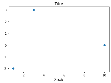
Matplotlib a un mode similaire à celui de Matlab, on enchaîne juste des appels à des fonctions pour réaliser des actions sur le même objet.
[115]:
plt.scatter([1, 3, 10], [-2, 3, 0])
plt.title("Titre")
plt.xlabel("X axis")
plt.savefig("comme_matlab.png")
[116]:
!comme_matlab.png
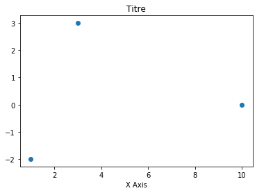
On va préférer la méthode par laquelle on modifier directement la figure au travers des objets qui la constituent.
[117]:
fig, ax = plt.subplots()
ax.scatter([1, 3, 10], [-2, 3, 0])
ax.set_title("Titre")
ax.set_xlabel("X Axis")
fig.savefig("avec_des_objets.jpg")
[118]:
!image_with_matplotlib.png
'image_with_matplotlib.png' n'est pas reconnu en tant que commande interne
ou externe, un programme ex‚cutable ou un fichier de commandes.
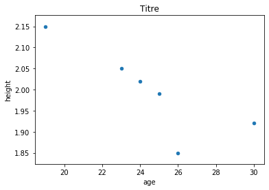
On peut utiliser Matplotlib directement mais on retrouve en fait la librairie un peu partout, dans pandas notamment.
[119]:
ax = df.plot(x="age", y="height", kind="scatter", title="Titre")
fig = ax.get_figure()
fig.savefig("avec_pandas.pdf")
[120]:
!avec_pandas.pdf
[67]:
!del /f comme_matlab.png avec_des_objets.jpg avec_pandas.pdf